
EDUCATION
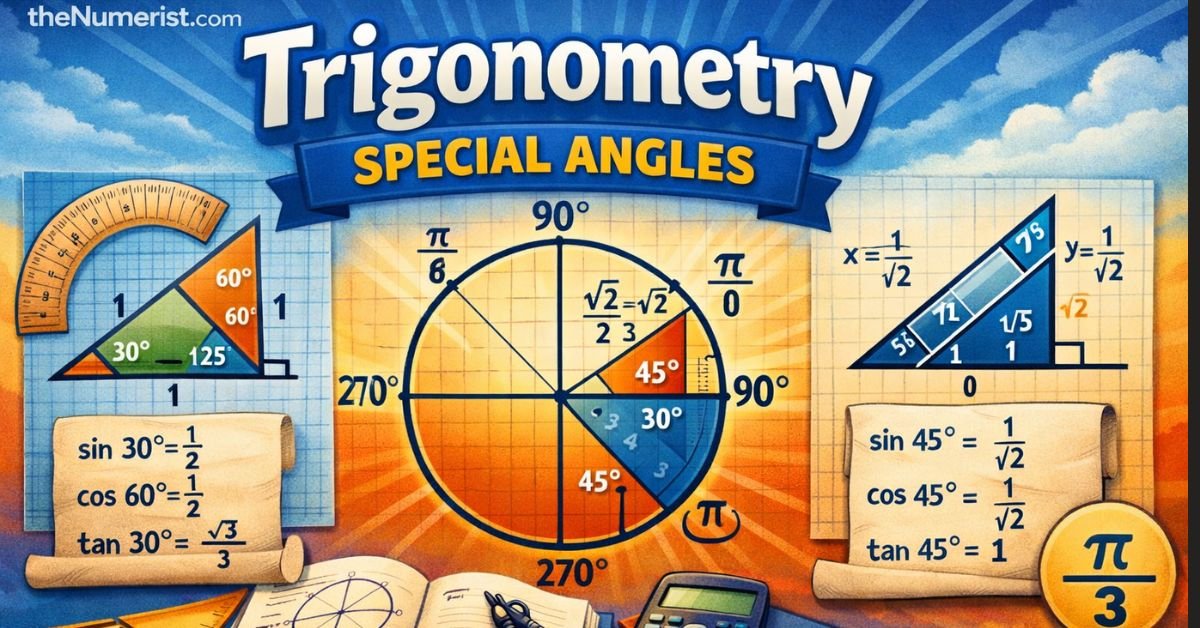
Trigonometry: Special Angle Triangles
Trigonometry is the type of math that you use when you want to work with angles. Luckily, some angles are used so frequently that they have their own dedicated name and shortcuts that you can memorize. These are called special angles in trigonometry, and you can use special angle triangles to help.
Special angles are great to know because their trigonometric functions equate to very specific and known ratios, so if you can memorize these it will save you a lot of time in doing trigonometry homework! To make things a bit easier, if you can’t remember these exact values, it is even easier to memorize the special angle triangles that these angles are based off of! And there are only two triangles, so you will find that it is very easy to derive the trig functions if you can’t remember them.
Specifically, the trig functions are easy to find for these special angles, which are: 0, 30, 45, 60, and 90 degrees.
45-45-90 Triangle
This will hopefully make sense after looking at the triangles I mentioned. Here’s another site that also talks about remembering the patterns of these triangles instead of specifically remembering the math. Create a right angle triangle with two 45 degree angles, and with two sides of 1 unit length. By using the Theorem of Pythagoras, you can find that the hypotenuse of this triangle is easy to calculate to be length √2. This is what this triangle looks like:
So then, from these values and using the memorization trick of SOHCAHTOA (here a quick trig cheat sheet for reference), you can obtain the trigonometric values for this special angle of 45 degrees. You can work out that:
Sin(45) = 1/√2
Cos(45) = 1/√2
Tan(45) = 1
Don’t worry if you can’t remember these values and ratios. The easiest way to remember them is to memorize how to construct the special angle triangle. And as you can see, this triangle is very simple: a right angle triangle with a 45 degree angle and 2 sides of length 1, and you can easily fill in the rest and then work out the ratios yourself.
30-60-90 Triangle
The second of the special angle triangles, which describes the remainder of the special angles, is slightly more complex, but not by much. Create a right angle triangle with angles of 30, 60, and 90 degrees. The lengths of the sides of this triangle are 1, 2, √3 (with 2 being the longest side, the hypotenuse. Make sure you don’t put the √3 as the hypotenuse!). FreeMathHelp also has a good explanation of this particular triangle. This triangle looks like this:
Here are the trig ratios that you can easily find:
Sin(30) = 1/2
Cos(30) = √3/2
Tan(30) = 1/√3
Sin(60) = √3/2
Cos(60) = 1/2
Tan(60) = √3/1 = √3
Once again, just remember the triangle, and the ratios are easy to derive!
For 0 and 90 degrees, there isn’t a triangle to remember (although please feel free to correct me if I am wrong!), so you will actually have to memorize these values. However, these aren’t complex. I usually just remember the pattern of the following list:
Sin(0) = 0
Cos(0) = 1
Tan(0) = 0
Sin(90) = 1
Cos(90) = 0
Tan(90) = undefined
If you can’t memorize the actual trigonometric ratios for the special angles, the key is to recall the special angle triangles that describe them. Make sure that you know how to construct the triangles, and then you can solve the trig ratios of the trigonometry special angles. You will quickly find that doing trigonometry questions that use these special angles are easy!
(This is an old post from my previous math site, In Mathematics, copied here to consolidate all my math pages.)

Shifting graphs horizontally (also known as horizontal translation) is slightly different from vertical translation, but still pretty straight-forward. Perhaps it would be helpful to review my posting on vertical shifts of graphs. Recall from that section: “Picture all the complex stuff that is happening to x as being one chunk of the height component, and then when you add the + 5 to the equation, you are really just adding an additional height chunk to the total height for a given x.” I think this simplification condenses the rest of that post down quite nicely.
Shifting Graphs – Horizontal Translation
Now, to shift a graph horizontally, you include the shift amount with x. So, whatever action was being done just to x before, now you do that same thing to x plus the shift amount. Make sense? Probably not.
Check out the example below that hopefully demonstrates this better than I can explain with words.
If you want to shift the original function of f(x) = x2 + 4 by 3 units, it becomes f(x) = (x-3)2 + 4.
Can you see what I mean by including the shift amount WITH x. The ‘square’ function acts on the entire (x-3) term. This will cause the graph to shift 3 units to the RIGHT. This may seem somewhat counter-intuitive, but it is correct. Subtracting terms from x shift the graph to the right, whereas adding terms to x will translate them to the left.
In this example, x-3 causes a horizontal translation of the graph 3 units right… if it were x+3, it would translate the graph 3 units left. Here is a bit of a trick you can use to help you recall the direction of the shift caused by the signs. It may be easier to remember this by analyzing the “x and shift amount”, letting this small term equal to 0, and then solving for x. The result will show you how many units to move, and in what direction. Like this:
x – 3 = 0
x = 3 (shift 3 units right)
OR
x + 3 = 0
x = (-3) (shift 3 units left)
That shows you how far over, and in what direction, the new x values are! Technically, this is a way of finding a zero of the graph, but that is another post for another day. For now, I think it’s a helpful trick to apply at this stage!
I hope these postings on graph manipulations are helpful. Horizontal translation of functions and their graphs is still quite simple, albeit with the trick with the signs that you don’t have to worry about with vertical translation.
ALSO READ: Using the Quadratic Formula

In this post, I’m going to explain a very frequently requested topic – how to convert your equation of a line from point-slope form to standard form. Sounds easy, right? Well, it isn’t difficult at all, provided that you understand the terminology and know what you’re doing. Follow along and hopefully all will become clear!
You are familiar with the general form of y=mx+b (also known as slope-intercept form), and you know that this equation tells you all that is necessary to actually graph this line – namely, the slope and y-intercept. However, what about if you have a section of your line up in quadrant I at the ordered pair coordinate of (150332, 23098)? The y-intercept on this graph doesn’t seem terribly useful way over here at this distant point! In this case, it’s probably more appropriate to use the point-slope form for your equation of a line. I need to explain this form first, before going on to show you how to convert from point-slope form to standard form equations.
In the most simple explanation that I know of, you can very easily derive the point-slope form from a very well known concept: the slope formula! Recall that slope is equal to rise over run. But what does that mean, in terms of mathematical symbols. Well, as I explained already in a previous post, this refers to the difference in the y values between two points, divided by the difference of the x values between those same two points. In formula form, you get something like this to define slope:

Now, to arrive at the point-slope form, all you need to do is a very simple rearrangement, as follows. Then, let the y2 and x2 just be x and y, and you are left with what you need to know:

Hopefully, you can see the manipulation that I did there. I simply multiplied both sides by the denominator, and then switched sides so that you could see the more conventional form of this equation of a line. The 1’s and 2’s aren’t particularly important – here, the y1 and x1 terms are simply referring to a specific point, whereas x and y refers to any point.
To actually use this equation, you have a few ways. In one way, you can substitute in the m value and a given coordinate that is on your line for the y1 and x1 terms, and then go from there to simplify or solve for another point. Secondly, you can use two separate points to calculate the slope (remember, this is essentially just a rearranged slope formula!) Either way, this form of the equation of a line is incredibly useful and handy to know. And thankfully, being able to derive it easily from the slope formula gives you an easy way to come up with it if you can’t seem to remember it exactly when you need it the most (on exams!).
So, now that you know what point-slope is, let me refer you back to my previous post about standard form graphing equations – because, now I’m going to explain to you how to convert from point-slope to standard form. This isn’t a terribly complicated process, though it is extremely important to get right, because when done correctly, both forms mathematically represent the same line on a graph. Though, if you make an error, you will likely wind up with a different line altogether. It is important to pay attention to what form of the equation of a line you are being asked to provide, and then it’s just a matter of doing some of these steps!
Point-Slope Form to Standard Form
Example: Express the following equation in standard form, and state the values for A, B, and C.

As a first point, I want you to realize that this example is very explicitly provided in point-slope form – to the letter! It won’t always be so! In any case, here is the basic strategy of what you want to do: get all of the x’s and y’s together on one side, and get the constants (i.e. no variables) over to the other side. Then, it’s just a matter of combining like terms and simplifying things wherever possible. Probably the most important thing to remember here is that you need to multiply what’s inside the brackets by the constant on the outside! This is far too easy a step to miss, but will completely mess you up!

Hopefully you can follow along with those steps! All it is really is a rearrangement of the terms, grouping the x’s and y’s together, and the constants alone. When you get it into the final form as I have shown, it is easy to simply read off the values for A (the coefficient in front of the x), B (the coefficient in front of the y), and C (the constant with no variable attached to it). In this case, A is 2, B is -1, and C is -10. Remember, no number in front of the y means a 1 is assumed, and since the standard form has a +, in this case, the minus means there is a -1.
Try another one, a bit harder this time?
Example: Express the following equation in standard form, and state the values for A, B, and C.
In this case, note that it isn’t immediately in point-slope form – I’ve reversed the left side terms. Of course, it’s a simple matter of just rearranging these, like so:

There, now that’s more appropriate. Next, we just follow the same steps that we did above: multiply through the brackets, and then group the x’s and y’s and isolate the constants. Easy, right? Let’s see what we get.

I did all of the adding and subtracting on one line this time, but I did the same steps as I outline above, and as you can see, I have a final answer expressed in standard form! If you were to stop here, and say that A is 2/3, B is 1, and C is 7, you would most definitely be correct. However, there is a convention that many teachers and professors follow, and that is to remove everything from the denominator, wherever possible. In other words, teachers don’t like fractions! So, how do we get rid of our fraction? You probably have already figured out where I’m going with this – you simply have to multiply everything on both side by 3, the denominator, to cancel it out. Doing so, you wind up with this final standard form graphing equation:

In this case, A is 2, y is 3, and C is 21. Another note – these coefficients are different from those we originally got, but the underlying math is all the same still. You can take both forms of our answers, create a table of values for each, and manually plot out the lines to prove that these indeed are the same lines, even though the equations look a bit different. You will probably agree that this version of the equation of the line just looks a lot nicer.
So, hopefully those few examples have properly explained to you the steps to consider when you have to convert point-slope form to standard form graphing equations. It’s not as difficult as it sounds, you just have to remember the points I’ve described in this post. In the next post, I’ll expand this concept to explain how slope-intercept form fits into all of this. Eventually, you won’t even recognize what form you are actually working with. You will just recognize what you need to do with the numbers to get the information that you need to solve your problem.
Thanks for reading this rather lengthy post! Please remember to subscribe or click on one of the Follow buttons on the right side of this page! I appreciate the support! And don’t forget, comments are always welcome if you need more explanations!

How many grams in a quarter pound, we need to understand the basics of units of measurement. A quarter pound is a unit of weight commonly used in the United States, while grams are a unit of weight in the metric system.
The Metric System
The metric system is a decimal-based system that is widely used around the world. It’s based on the gram, which is a unit of weight that is defined as one thousandth of a kilogram.
Converting Quarter Pounds to Grams
To convert a quarter pound to grams, we need to know that 1 pound is equal to 453.592 grams. Therefore, a quarter pound is equal to 113.398 grams.

Practical Applications
Understanding how to convert between units of measurement is crucial in various fields, including cooking, science, and commerce. For instance, if you’re a recipe developer, you may need to convert ingredients from one unit to another to ensure accuracy.
One user reported, “I was trying to follow a recipe that used metric measurements, but I only had a scale that measured in pounds. I was able to convert the ingredients using an online converter, and it worked perfectly!”
Frequently Asked Questions
Q: How many grams are in a quarter pound?
A: A quarter pound is equal to 113.398 grams.
Q: How do I convert pounds to grams?
A: To convert pounds to grams, you can multiply the number of pounds by 453.592.
Q: What is the difference between a quarter pound and 100 grams?
A: A quarter pound is approximately 113.398 grams, which is more than 100 grams.
Q: Can I use an online converter to convert quarter pounds to grams?
A: Yes, there are many online converters available that can help you convert quarter pounds to grams quickly and accurately.
Conclusion
Units of measurement, you’ll discover the importance of understanding how to convert between different units. Whether you’re a professional or simply someone who loves to cook, being able to convert quarter pounds to grams is a valuable skill.
-

 TECH9 months ago
Apple iPhone 17: Official 2025 Release Date Revealed
-

 BLOG9 months ago
Understanding the ∴ Symbol in Math
-

 ENTERTAINMENT7 months ago
What Is SUV? A Family-Friendly Vehicle Explained
-

 EDUCATION4 weeks ago
Horizontal Translation: How to Shift Graphs
-

 EDUCATION9 months ago
Using the Quadratic Formula
-

 ENTERTAINMENT9 months ago
Going Live: How to Stream on TikTok from Your PC
-

 TECH9 months ago
Prodigy: Early Internet Pioneer
-

 EDUCATION9 months ago
The Meaning of an Open Circle in Math Explained